A Control-Theory Taxonomy of Physical AI
The Creation of Physical AI
As I walk down Mission St. in SF, I see a giant billboard: Michelangelo’s Creation of Adam, except instead of Adam’s hand reaching for God’s, it’s a robotic prosthetic reaching for the words “Physical AI.” Now it’s official: the Physical AI hype is on.
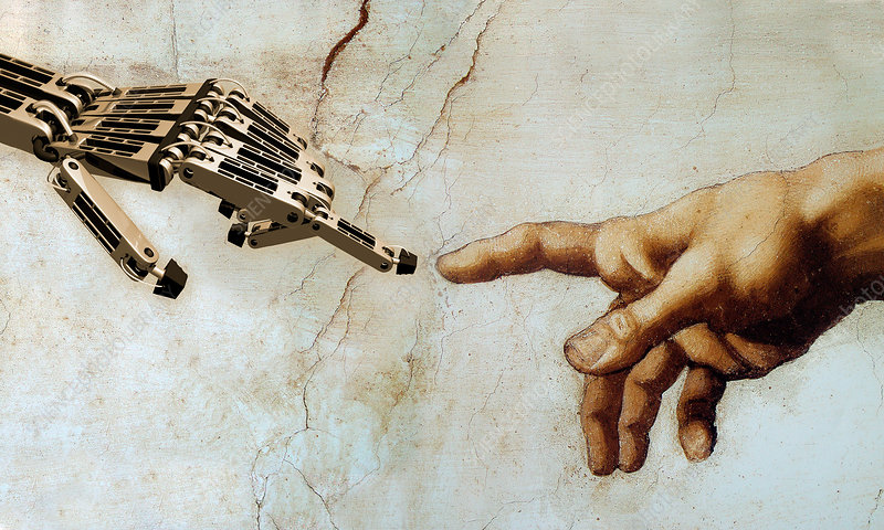
Fig. 1 — The Creation of Physical AI: the hype is on.1
When the term “Physical AI” appeared, I assumed it referred to AI for physics. But since then, it has come to include pretty much anything that touches the physical world: hardware, materials, robotics, biotech, world models, etc. All of it is Physical AI now. Given how overloaded the term has become, it’s worth asking what ties all of this together, and how.
This article explores the characteristics that define Physical AI methods and organizes them under the quintessential physical framework: control theory.2
How Is Physical Different from Non-Physical AI?
Let’s begin by defining what differentiates Physical from non-Physical AI.
- Physics constraints. The first and probably most accepted characteristic is that Physical AI must respect the governing equations of physics. A model trained on simulated or observed data must transfer to reality while still adhering to physics. There’s no room for hallucinations in Physical AI.
- Data scarcity and the sim-to-real gap. Physical AI data is often scarce. Unlike LLMs, which can rely on nearly unlimited text, physical experiments are slow and expensive. Manufacturing and measuring PCBs can take weeks; growing and sequencing cells can take months. Simulation can accelerate data collection, but it comes with the problem of alignment to reality. Calibrating a simulator can be difficult, and at times impossible. Since physical data is rare and expensive, Physical AI models must learn in limited data regimes while staying flexible enough to transfer to the real world.
- Sensing, embodiment, and the real-time closed loop. As living beings experience reality through different senses, Physical AI systems are expected to handle data from different sensors and modalities (e.g., vision, lidar, force, temperature). Physical AI continuously operates in the real world, and it is expected to behave as a closed-loop system.
This closed loop is exactly what control theory was built to capture, and it gives us a natural taxonomy for Physical AI itself.
A Taxonomy from the Control Loop
Control theory provides a clean framework for physical systems: a system senses its state, decides on an action, and acts in order to optimize some cost function.
Fig. 2 — Mapping Physical AI to closed-loop control. Illustration of a closed-loop control system consisting of set point w(t), measured output ym(t), measured error e(t), controller output u(t), system input us(t), disturbance d(t), and system output y(t). Colored blocks show where each Physical AI branch operates within the loop.
This naturally fits Physical AI methods that can be grouped into four categories mapping onto this same loop.
- Perception estimates the physical states from raw observations, taking in sensor data (e.g., camera, lidar, force, chemical) and turning them into state representations. This is the territory of computer vision, depth estimation, and state estimation.
- Model characterizes how the system and the world evolve. It learns physical dynamics, taking state and action as input and predicting future states. Neural operators, PINNs, surrogate models, and digital twins all fall under this group.
- Control addresses what the system should do next. Given the current state, it decides on and executes an action in real time. This is where policy learning, reinforcement learning, and optimal control live.
- Optimize determines what configuration achieves the goal. Starting from a target, it searches for or designs a solution with the desired properties. This is the domain of Bayesian optimization, inverse design, and generative design.
Tab. 1 — Physical AI architectures mapped to the Perception–Control–Model–Optimize taxonomy. The table is illustrative rather than comprehensive: entries are representative examples of each combination, not an exhaustive catalog. Hover over a block to see seminal papers.
The building blocks of this taxonomy are methods that sit within a single category. For instance, state estimation and vision models in Perception (ViT, SAM, DINO, YOLO); policy learning methods in Control (Diffusion Policy, ACT, BESO); surrogate models in Model (Neural ODE, GNS, GraphCast); and Bayesian optimization in Optimize (GP, TuRBO, SAASBO).
More flexible approaches spanning two branches are architectures that live at the Model–Optimize boundary (e.g., PINNs, Neural Operators, and Generative Design models), each capable of running forward as a surrogate or backward as an inverse solver; or VLAs, which blend Perception and Control into a single model (e.g., GR00T, RT-2, π₀).
Finally, World Models (e.g., Cosmos, DreamerV3, JEPA) span three categories, blending Perception, Model, and Control entirely in latent space. They encode observations, predict future states, and plan over imagined solutions without interacting with the real world.
This taxonomy brings some order to the crowded Physical AI space where methods that rarely appear in the same conversation all find a place under the same umbrella. This table also highlights that a fundamental difference between control theory and Physical AI is that AI models allow us to cross boundaries between functional categories. For instance, classical robotic stacks maintain separate vision, state estimation, and policy modules while a VLA collapses them into a single model. Similarly, PINNs are capable of both modeling dynamical systems and solving inverse problems depending on the direction in which a model is queried.
Reaching for the Fourth Column
A pattern emerges from the proposed framework. Classical techniques sit in a single column. More recent methods occupy two columns: PINNs run forward as surrogates and backward as inverse solvers, VLAs merge Perception and Control. World Models cover three columns. The extrapolated question is then: is a four column model next? A single foundation model that perceives, models, controls, and optimizes. Self-driving labs3 and auto-research4,5 are some of the closest examples we have today: systems that propose a design, run experiments, observe results, and decide what to try next.
However, to the best of my knowledge, neither is quite there. Self-driving labs don’t yet run on a single model, but on a combination of specialized ones stitched together. And auto-research hasn’t yet made direct contact with the physical world.
And this is where Physical AI stands. The robotic hand is reaching but the fingers haven’t met yet. Physical heaven is still a few centimeters away.
Creation of Robotic Adam, Science Photo Library. sciencephoto.com/media/92834.
K.J. Åström and R.M. Murray, Feedback Systems: An Introduction for Scientists and Engineers, Princeton University Press, 2nd ed., 2021.
N.J. Szymanski et al., An autonomous laboratory for the accelerated synthesis of novel materials, Nature 624, 86–91, 2023. nature.com/articles/s41586-023-06734-w.
A. Novikov et al., AlphaEvolve: A coding agent for scientific and algorithmic discovery, Google DeepMind, 2025. deepmind.google.
A. Karpathy, autoresearch, 2026. github.com/karpathy/autoresearch.